build:
cran:
doi:
github:

Vehicular Emissions INventories (VEIN)

TODO

Include speed functions with Fortran
Include CB6
Add EF from HBEFA?
See issues GitHub

System requirements

vein imports functions from spatial packages listed below. In order to install these packages, firstly the user must install the requirements mentioned here.

Installation

CRAN

VEIN can be installed via CRAN or github

install.packages("vein")

GitHub

remotes::install_github("atmoschem/vein")

or if you have a 32 bits machine

install_github("atmoschem/vein",
INSTALL_opts = "--no-multiarch")

demo

Then, if you want, run the demo

library(vein) 
demo(VEIN)

Approaches

1. get a project (easier)

At the moment, most of the projects covers Brazilian regions, but I will include China, Europe or USA approaches as soon as I can.

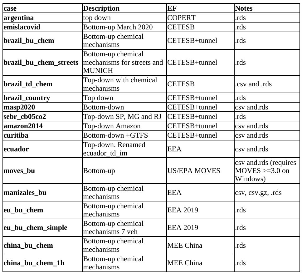
Use the function get_project and read the documentation, there you can see more projects as well.

Check the projects here: (https://atmoschem.github.io/vein/reference/get_project.html)[https://atmoschem.github.io/vein/reference/get_project.html]

library(vein)
?get_project
get_project(directory = "awesome_city")

The structure of the new directory “awesome_city” is:

awesome_city
├── config
│   ├── clean.R
│   ├── config.R
│   ├── inventory.xlsx
│   └── packages.R
├── main.R
├── main.Rproj
├── network
│   ├── net.gpkg
│   └── net.rds
├── scripts
│   ├── evaporatives.R
│   ├── exhaust.R
│   ├── fuel_eval.R
│   ├── net.R
│   ├── pavedroads.R
│   ├── plots.R
│   ├── post.R
│   ├── traffic.R
│   └── wrf.R
└── wrf
└── wrfinput_d02

You have to open the file main.Rproj with Rstudio and then open and run main.R

To run main.R you will need these extra packages:

ggplot2
readxl
eixport (If you plan to generate WRF Chem emissions file)

If you do not have them already, you can install:

install.packages(c("ggplot2", "readxl", "eixport"))

Too complicated? Watch a YouTube

English

Portuguese

2. Use inventory (a bit not so easy)

Read the instruction of inventory

?inventory

1) Examples with traffic data:

If you know the distribution of the vehicles by age of use , use: my_age
If you know the sales of vehicles or better the registry of new vehicles, use age to apply a survival function.
If you know the theoretical shape of the circulating fleet and you can use age_ldv, age_hdv or age_moto. For instance, you dont know the sales or registry of vehicles, but somehow you know the shape of this curve.
You can use/merge/transform/adapt any of these functions.

library(vein)
data("net")
PC_E25_1400 <- age_ldv( x = net$ldv)

plot(PC_E25_1400)
#> Weighted mean =  11.17

If you want to know the vehicles per street and by age of use, just add the net. Age functions now returns ‘sf’ objects if the net argument is present.

PC_E25_1400net <- age_ldv(
  x = net$ldv, 
  net = net
)
plot(PC_E25_1400net, 
  key.pos = 4, 
  pal = cptcity::cpt(
    colorRampPalette = T, 
    rev = T))
#> old-style crs object detected; please recreate object with a recent sf::st_crs()
#> old-style crs object detected; please recreate object with a recent sf::st_crs()
#> Warning: plotting the first 9 out of 50 attributes; use max.plot = 50 to plot
#> all
#> old-style crs object detected; please recreate object with a recent sf::st_crs()
#> old-style crs object detected; please recreate object with a recent sf::st_crs()
#> old-style crs object detected; please recreate object with a recent sf::st_crs()
#> old-style crs object detected; please recreate object with a recent sf::st_crs()
#> old-style crs object detected; please recreate object with a recent sf::st_crs()
#> old-style crs object detected; please recreate object with a recent sf::st_crs()
#> old-style crs object detected; please recreate object with a recent sf::st_crs()
#> old-style crs object detected; please recreate object with a recent sf::st_crs()
#> old-style crs object detected; please recreate object with a recent sf::st_crs()
#> old-style crs object detected; please recreate object with a recent sf::st_crs()
#> old-style crs object detected; please recreate object with a recent sf::st_crs()
#> old-style crs object detected; please recreate object with a recent sf::st_crs()
#> old-style crs object detected; please recreate object with a recent sf::st_crs()
#> old-style crs object detected; please recreate object with a recent sf::st_crs()
#> old-style crs object detected; please recreate object with a recent sf::st_crs()
#> old-style crs object detected; please recreate object with a recent sf::st_crs()
#> old-style crs object detected; please recreate object with a recent sf::st_crs()
#> old-style crs object detected; please recreate object with a recent sf::st_crs()
#> old-style crs object detected; please recreate object with a recent sf::st_crs()
#> old-style crs object detected; please recreate object with a recent sf::st_crs()
#> old-style crs object detected; please recreate object with a recent sf::st_crs()
#> old-style crs object detected; please recreate object with a recent sf::st_crs()
#> old-style crs object detected; please recreate object with a recent sf::st_crs()
#> old-style crs object detected; please recreate object with a recent sf::st_crs()
#> old-style crs object detected; please recreate object with a recent sf::st_crs()
#> old-style crs object detected; please recreate object with a recent sf::st_crs()
#> old-style crs object detected; please recreate object with a recent sf::st_crs()
#> old-style crs object detected; please recreate object with a recent sf::st_crs()
#> old-style crs object detected; please recreate object with a recent sf::st_crs()
#> old-style crs object detected; please recreate object with a recent sf::st_crs()
#> old-style crs object detected; please recreate object with a recent sf::st_crs()
#> old-style crs object detected; please recreate object with a recent sf::st_crs()
#> old-style crs object detected; please recreate object with a recent sf::st_crs()
#> old-style crs object detected; please recreate object with a recent sf::st_crs()
#> old-style crs object detected; please recreate object with a recent sf::st_crs()
#> old-style crs object detected; please recreate object with a recent sf::st_crs()
#> old-style crs object detected; please recreate object with a recent sf::st_crs()
#> old-style crs object detected; please recreate object with a recent sf::st_crs()

temporal factors and netspeed

data("net")
data("pc_profile")
pc_week <- temp_fact(
  net$ldv + net$hdv, 
  pc_profile
)
dfspeed <- netspeed(
  q = pc_week, 
  ps = net$ps, 
  ffs = net$ffs, 
  cap = net$capacity, 
  lkm = net$lkm, 
  alpha = 1.5
)
plot(dfspeed)
#> Weighted mean =  44.16

If you want ot check the speed at different hours by street, just add net:

dfspeednet <- netspeed(
  q = pc_week, 
  ps = net$ps, 
  ffs = net$ffs, 
  cap = net$capacity, 
  lkm = net$lkm,
  alpha = 1.5, 
  net = net
)
plot(
  dfspeednet[, c("S1", "S9")], 
  key.pos = 4, 
  pal = cptcity::cpt(colorRampPalette = T, 
                     rev = T), 
  axes = T
)
#> old-style crs object detected; please recreate object with a recent sf::st_crs()
#> old-style crs object detected; please recreate object with a recent sf::st_crs()
#> old-style crs object detected; please recreate object with a recent sf::st_crs()
#> old-style crs object detected; please recreate object with a recent sf::st_crs()
#> old-style crs object detected; please recreate object with a recent sf::st_crs()
#> old-style crs object detected; please recreate object with a recent sf::st_crs()
#> old-style crs object detected; please recreate object with a recent sf::st_crs()
#> old-style crs object detected; please recreate object with a recent sf::st_crs()
#> old-style crs object detected; please recreate object with a recent sf::st_crs()
#> old-style crs object detected; please recreate object with a recent sf::st_crs()
#> old-style crs object detected; please recreate object with a recent sf::st_crs()
#> old-style crs object detected; please recreate object with a recent sf::st_crs()
#> old-style crs object detected; please recreate object with a recent sf::st_crs()
#> old-style crs object detected; please recreate object with a recent sf::st_crs()
#> old-style crs object detected; please recreate object with a recent sf::st_crs()
#> old-style crs object detected; please recreate object with a recent sf::st_crs()

#### 2) Emission Factors

V <- 0:150
ef1 <- ef_ldv_speed(
  v = "PC",
  t = "4S", 
  cc = "<=1400", 
  f = "G",
  eu = "PRE",
  p = "CO"
)
ef2 <- ef_ldv_speed(
  v = "PC",
  t = "4S", 
  cc = "<=1400", 
  f = "G",
  eu = "III",
  p = "CO"
)

ef1 <- EmissionFactors(ef1(1:150))
ef2 <- EmissionFactors(ef2(1:150))
colplot(data.frame(PRE = ef1, III = ef2))

3) Estimation of emissions

emis

euro <- c(
  rep("V", 5), 
  rep("IV", 5), 
  rep("III", 5), 
  rep("II", 5),
  rep("I", 5), 
  rep("PRE", 15)
)
lef <- lapply(1:40, function(i) {
  ef_ldv_speed(
    v = "PC", 
    t = "4S",
    cc = "<=1400", 
    f = "G",
    eu = euro[i], 
    p = "CO", 
    show.equation = FALSE
  ) 
})
E_CO <- emis(
  veh = PC_E25_1400, 
  lkm = net$lkm, 
  ef = lef, 
  speed = dfspeed,
  profile = pc_profile
)

4) Post Emissions

emis_post
When the argument by = “veh” the emissions are aggregated by age and hour.
When the argument by = “streets_wide”, aggregated the emissions by street. In this cae, if you add the argument net with the respective streets, it returns an spatial net with the hourly emissions.

E_CO_DF <- emis_post(
  arra = E_CO,  
  veh = "PC", 
  size = "<1400", 
  fuel = "G",
  pollutant = "CO", 
  by = "veh", 
  type_emi = "exhaust"
)
E_CO_STREETS <- emis_post(
  arra = E_CO, 
  pollutant = "CO", 
  by = "streets", 
  net = net
)
plot(
  E_CO_STREETS[, c("V1", "V9")], 
  key.pos = 4, 
  pal = cptcity::cpt(colorRampPalette = T, 
                     rev = T), 
  axes = T)
#> old-style crs object detected; please recreate object with a recent sf::st_crs()
#> old-style crs object detected; please recreate object with a recent sf::st_crs()
#> old-style crs object detected; please recreate object with a recent sf::st_crs()
#> old-style crs object detected; please recreate object with a recent sf::st_crs()
#> old-style crs object detected; please recreate object with a recent sf::st_crs()
#> old-style crs object detected; please recreate object with a recent sf::st_crs()
#> old-style crs object detected; please recreate object with a recent sf::st_crs()
#> old-style crs object detected; please recreate object with a recent sf::st_crs()
#> old-style crs object detected; please recreate object with a recent sf::st_crs()
#> old-style crs object detected; please recreate object with a recent sf::st_crs()
#> old-style crs object detected; please recreate object with a recent sf::st_crs()
#> old-style crs object detected; please recreate object with a recent sf::st_crs()
#> old-style crs object detected; please recreate object with a recent sf::st_crs()
#> old-style crs object detected; please recreate object with a recent sf::st_crs()
#> old-style crs object detected; please recreate object with a recent sf::st_crs()
#> old-style crs object detected; please recreate object with a recent sf::st_crs()

Grids

make_grid.

Create a grid using make_grid.The spobj is the spatial net. The size of the grid has the size of the net. You have to specify the grid spacing.
Create a grid using a path to wrfinput file instead a net. The grid will have the size of the wrf_input. You don’t have to specify the grid spacing.

data(net)
E_CO_STREETSnet <- emis_post(
  arra = E_CO, 
  pollutant = "CO",
  by = "streets_wide",
  net = net
)
g <- make_grid(
  spobj = net, 
  width = 1/102.47
)
#> old-style crs object detected; please recreate object with a recent sf::st_crs()
#> old-style crs object detected; please recreate object with a recent sf::st_crs()
#> Number of lon points: 12
#> Number of lat points: 10
#> old-style crs object detected; please recreate object with a recent sf::st_crs()
E_CO_g <- emis_grid(
  spobj = E_CO_STREETSnet, 
  g = g, 
  sr= 31983
)
#> Your units are:
#> g
#> Transforming spatial objects to 'sr'
#> old-style crs object detected; please recreate object with a recent sf::st_crs()
#> Sum of street emissions 148791715.29
#> Sum of gridded emissions 148791715.29
na <- paste0("V", 1:168)
for(i in 1:168) E_CO_g[[na[i]]] <- E_CO_g[[na[i]]] * units::set_units(1, "1/h")
plot(
  E_CO_g[, c("V1", "V9")], 
  key.pos = 4, 
  pal = cptcity::cpt(colorRampPalette = T, 
                     rev = T,
                     pal = "mpl_viridis"), 
  axes = T, 
  lty = 0
)

Creating a WRFChem Input file using eixport:

Create a grid using make_grid and a wrfinput file
Run emis_grid to grid your emissions.
Create a GriddedEmissionsArray.
Create a wrfchem input file [eixport::wrf_create](https://atmoschem.github.io/eixport/reference/wrf_create.html.
Put the GriddedEmissionsArray into the wrf chem input file using eixport::wrf_put.

library(eixport)
dir.create(file.path(tempdir(), "EMISS"))
wrf_create(wrfinput_dir         = system.file("extdata", package = "eixport"),
wrfchemi_dir         = file.path(tempdir(), "EMISS"),
domains              = 2,
frames_per_auxinput5 = 1, #hours
auxinput5_interval_m = 60,
verbose              = TRUE)
path_to_wrfi <- paste0(system.file("extdata", package = "eixport"), "/wrfinput_d02")
path_to_wrfc <- list.files(file.path(tempdir(), "EMISS"), full.names = TRUE)[1]
gwrf <- eixport::wrf_grid(path_to_wrfi)
E_CO_gwrf <- emis_grid(spobj = E_CO_STREETSnet, g = gwrf)
gr <- GriddedEmissionsArray(E_CO_gwrf, rows = 51, cols = 63, times = 1)
eixport::wrf_put(file = path_to_wrfc, name = "E_CO", POL = gr)

Creating a WRFChem Input file using AS4WRF

Create a grid using make_grid and your net.
Run emis_grid to grid your emissions.
Run eixport::to_as4wrf to create a data.frame the specifications for AS4WRF.ncl.
Export data.frame to a text.file. Recall that AS4WRF requires all the lumped species.
Contact the developer of AS4WRF Angel Vara alvv1986@gmail.com to get a copy and run AS4WRF.ncl.

Thanks and enjoy VEIN!

Citation

If you use VEIN, please, cite it (BIBTEX, ENDNOTE):

Ibarra-Espinosa, S., Ynoue, R., O’Sullivan, S., Pebesma, E., Andrade, M. D. F., and Osses, M.: VEIN v0.2.2: an R package for bottom-up vehicular emissions inventories, Geosci. Model Dev., 11, 2209-2229, https://doi.org/10.5194/gmd-11-2209-2018, 2018.

@article{gmd-11-2209-2018,
author = {Ibarra-Espinosa, S. and Ynoue, R. and O'Sullivan, S. and Pebesma, E. and Andrade, M. D. F. and Osses, M.},
title = {VEIN v0.2.2: an R package for bottom--up vehicular emissions inventories},
journal = {Geoscientific Model Development},
volume = {11},
year = {2018},
number = {6},
pages = {2209--2229},
url = {https://gmd.copernicus.org/articles/11/2209/2018/},
doi = {10.5194/gmd-11-2209-2018}
}

Special thanks to all the contributors

Communications, doubts etc

Earth-Sciences on Stackoverflow, tag vein-r-package
Drop me an email sergio.ibarra@usp.br or zergioibarra@hotmail.com (你好中国朋友 - Hello Chinese friends!)
Check the group on GoogleGroups Group.
Check the project on ResearchGate.

Issues

If you encounter any issues while using VEIN, please submit your issues to: https://github.com/atmoschem/vein/issues/ If you have any suggestions just let me know to sergio.ibarra@usp.br.

Contributing

Please, read this guide. Contributions of all sorts are welcome, issues and pull requests are the preferred ways of sharing them. When contributing pull requests, please follow the Google’s R Style Guide. This project is released with a Contributor Code of Conduct. By participating in this project you agree to abide by its terms.

Note for non-english and anaconda users

Sometimes you need to install R and all dependencies and a way for doing that is using anaconda. Well, as my system is in portuguese, after installing R using anaconda it changed the decimal character to ‘,’. In order to change it back to english meaning decimal separator as ‘.’, I added this variable into the .bashrc

nano ~/.bashrc
export Lang=C

More details on StackOverflow

VEIN

Vehicular Emissions INventories (VEIN)

TODO

System requirements

Installation

CRAN

GitHub

demo

Approaches

1. get a project (easier)

Too complicated? Watch a YouTube

2. Use inventory (a bit not so easy)

1) Examples with traffic data:

3) Estimation of emissions

4) Post Emissions

Grids

Creating a WRFChem Input file using eixport:

Creating a WRFChem Input file using AS4WRF

Citation

Special thanks to all the contributors

Communications, doubts etc

Issues

Contributing

Note for non-english and anaconda users

Links

License

Community

Citation

Developers