plot WRF: Elevation

Here we attempt to provide useful code to generate figures from WRF outputs based on known galleries. For instance, NCL and WRF-Python provides extensive examples for plotting WRF outputs. Therefore, we aim to replicate some of these. Our approach to read wrfout files is based on eixport which relies r packages with GDAL bindings such as raster and stars. We do not try to provide a full gallery, instead, some basics and necessary plots to inspire other R used and receive more examples so share with the community.

packages

eixport read and manipulate wrf files.
raster for gridded and raster data.
stars for gridded and raster data.
cptcity colour palettes.
sf for spatial vector data.

library(eixport)
library(raster)
#> Loading required package: sp
library(stars)
#> Loading required package: abind
#> Loading required package: sf
#> Linking to GEOS 3.12.1, GDAL 3.8.4, PROJ 9.4.0; sf_use_s2() is TRUE
library(cptcity)
library(sf)

Based on NCL:

wrfo <- "/home/sergio/R/x86_64-pc-linux-gnu-library/4.3/helios/extras/wrfout_d01_2020-01-01_01%3A00%3A00_sub.nc"

Reading T2 from wrfout

T2 <- wrf_get(wrfo,  "T2", as_raster = T)
T2 <- T2[[1]] # by default one variable with each time, so we select one

Adding coastlines and cropping for our study area

library(rnaturalearth)
cl <- ne_countries(scale = "small", returnclass = "sf")
cl <- st_transform(cl, 31983)
T2 <- st_transform(st_as_stars(T2), 31983)
cl <- st_cast(st_crop(cl, T2), "LINESTRING")
#> Warning: attribute variables are assumed to be spatially constant throughout
#> all geometries
#> Warning in st_cast.sf(st_crop(cl, T2), "LINESTRING"): repeating attributes for
#> all sub-geometries for which they may not be constant

Find colour palette for elevation

find_cpt("elevation")
#> [1] "gmt_GMT_elevation" "grass_elevation"

#spplot(HGT, main = "HGT using spplot", scales=list(draw = TRUE),
#       col.regions = cpt("grass_elevation"),
#       sp.layout = list("sp.lines", as_Spatial(cl), col = "black"))

cols <- classInt::classIntervals(T2[[names(T2)]], 
                                 n = 100, 
                                 style = "pretty")
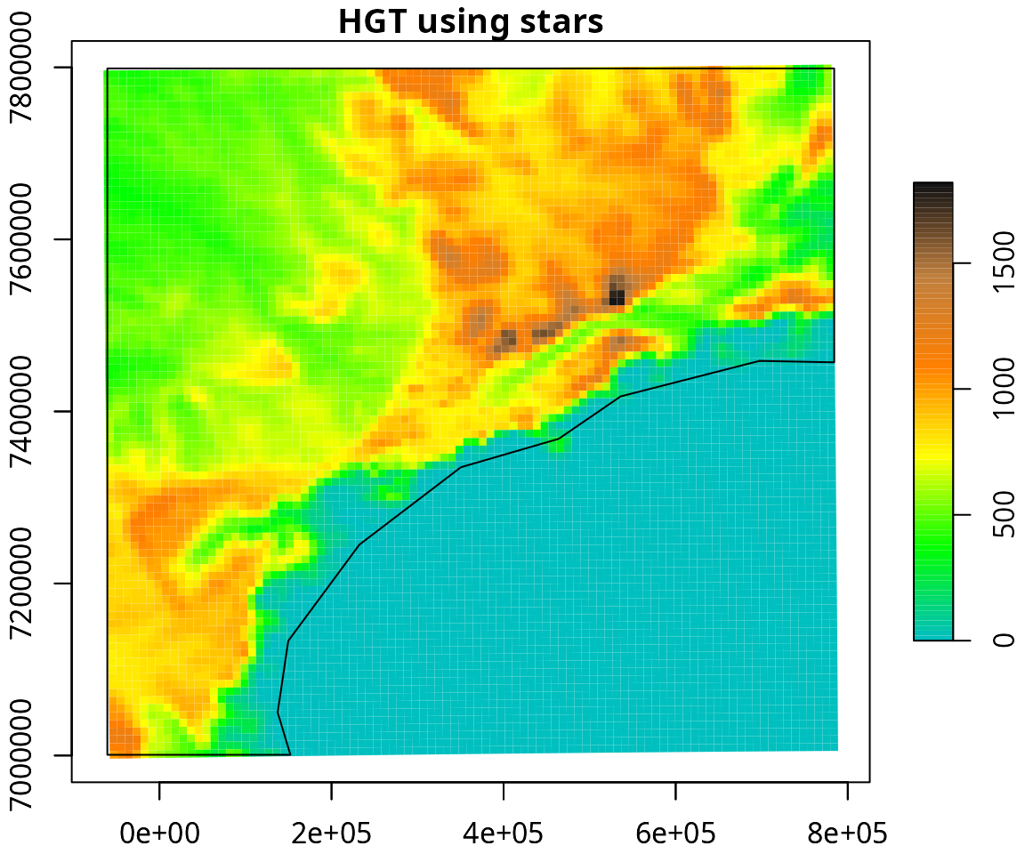
plot(T2, axes = T, main = "HGT using stars", col = cpt("grass_elevation", n = length(cols$brks) - 1), breaks = cols$brks, reset = F)
plot(cl$geometry, add= T, col = "black")

Sergio Ibarra-Espinosa

2024-09-22

packages