plot WRF: Cross sections

Based on this NCL

library(eixport)
library(raster)
#> Loading required package: sp
library(stars)
#> Loading required package: abind
#> Loading required package: sf
#> Linking to GEOS 3.12.1, GDAL 3.8.4, PROJ 9.4.0; sf_use_s2() is TRUE
library(cptcity)
library(sf)
library(vein)
library(ggplot2)

Reading Temperature and crop coast lines for our study area

wrfo <- "/home/sergio/R/x86_64-pc-linux-gnu-library/4.3/helios/extras/wrfout_d01_2020-01-01_01%3A00%3A00_sub.nc"
t2 <- mean(wrf_get(wrfo, "T2", as_raster = T))
t2[] <- t2[] -273.15# we select one

Find colour palette for temperature

find_cpt("temperature")
#> [1] "arendal_temperature"    "idv_temperature"        "jjg_misc_temperature"  
#> [4] "kst_03_red_temperature"

Let us create a line between c(-46.5,-23.85) and c(-46.35, -23.95)

cx <- as.data.frame(coordinates(projectRaster(t2, crs="+proj=longlat")))

m <- cbind(c(min(cx$x),  # xini
             max(cx$y)), # xend
           c(min(cx$y),  # yini
             max(cx$y))) # yend
cross = st_linestring(m)
(cross <- st_sfc(cross, crs = 4326))
#> Geometry set for 1 feature 
#> Geometry type: LINESTRING
#> Dimension:     XY
#> Bounding box:  xmin: -120.0101 ymin: 37.72342 xmax: 39.52542 ymax: 39.52542
#> Geodetic CRS:  WGS 84
#> LINESTRING (-120.0101 37.72342, 39.52542 39.52542)
plot(mean(t2), 
     main = "Temperature using plot", 
     col = cpt("arendal_temperature"))
plot(cross, add = T)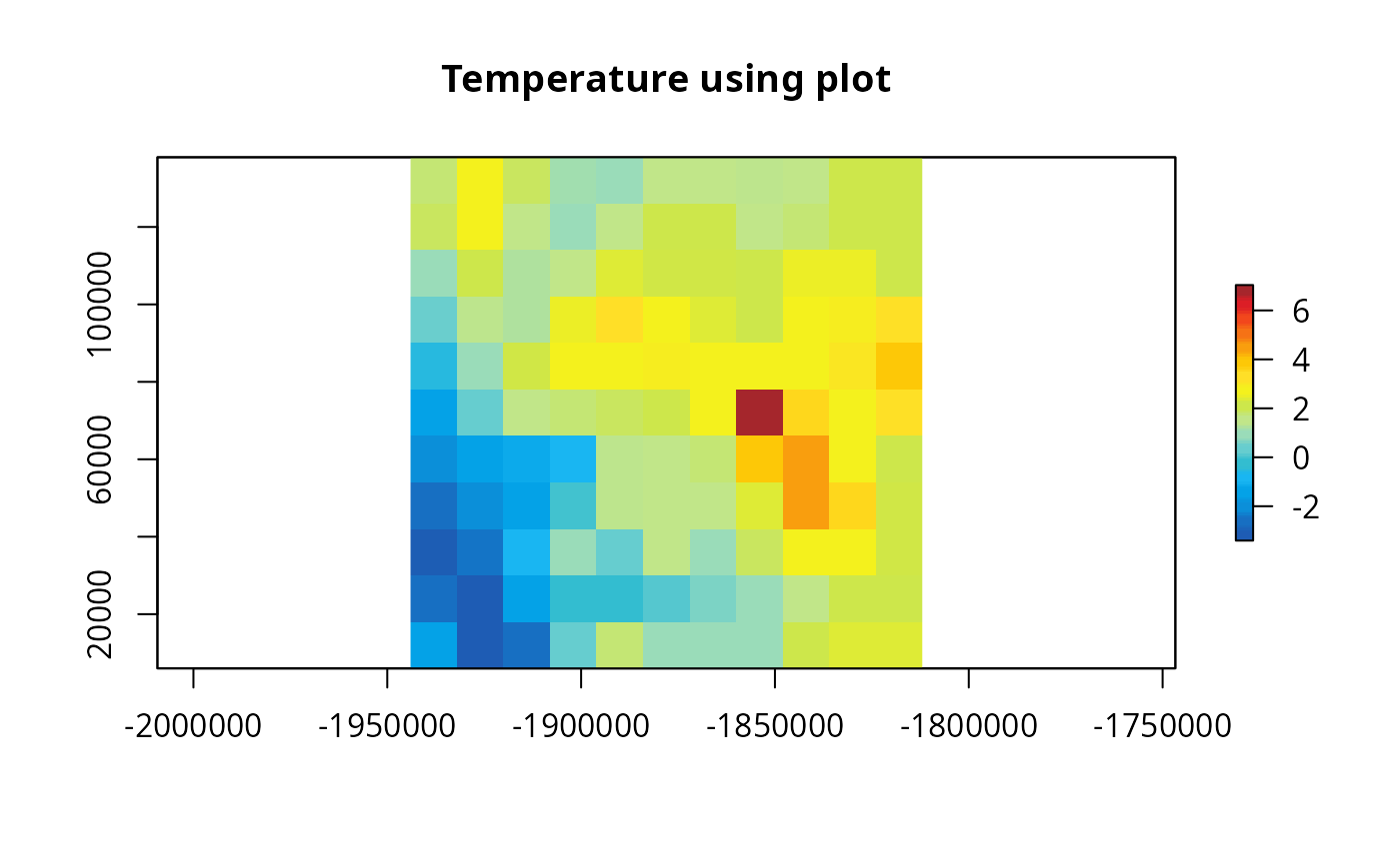

Define a helper function

points_extract <- function(m, sta) {
  cross = st_linestring(m)
  cross <- st_sfc(cross, crs = 4326)
  t2s <- st_as_sf(sta)
  lt <- st_intersection(t2s, cross) 
  geo <- st_geometry(lt)
  lt <- st_set_geometry(lt, NULL)
  na <- names(lt)
  lt$id <- 1:nrow(lt)
  dx <- vein::wide_to_long(df = lt, 
                           column_with_data = na, 
                           column_fixed = "id")
  stf <- st_sf(dx, geometry = geo)
  lt <- st_centroid(stf)
  lt <- cbind(lt, st_coordinates(lt))
  
  return(lt)
}

sta = st_as_stars(t2)
sta <- st_transform(sta, 4326)
names(sta) <- "temperature"
df <- points_extract(m, sta = sta)
#> Warning: attribute variables are assumed to be spatially constant throughout
#> all geometries
#> Warning: st_centroid assumes attributes are constant over geometries

Let us check the data

head(df)
#> Simple feature collection with 6 features and 5 fields
#> Geometry type: POINT
#> Dimension:     XY
#> Bounding box:  xmin: -119.6334 ymin: 38.75301 xmax: -119.4923 ymax: 39.13083
#> Geodetic CRS:  WGS 84
#>         V1 V2          V3         X        Y                   geometry
#> 1 1.885952  1 temperature -119.5149 39.07052 POINT (-119.5149 39.07052)
#> 2 1.123045  2 temperature -119.4923 39.13083 POINT (-119.4923 39.13083)
#> 3 1.602649  3 temperature -119.5434 38.99434 POINT (-119.5434 38.99434)
#> 4 1.978644  4 temperature -119.5991 38.84526 POINT (-119.5991 38.84526)
#> 5 1.229632  5 temperature -119.5766 38.90559 POINT (-119.5766 38.90559)
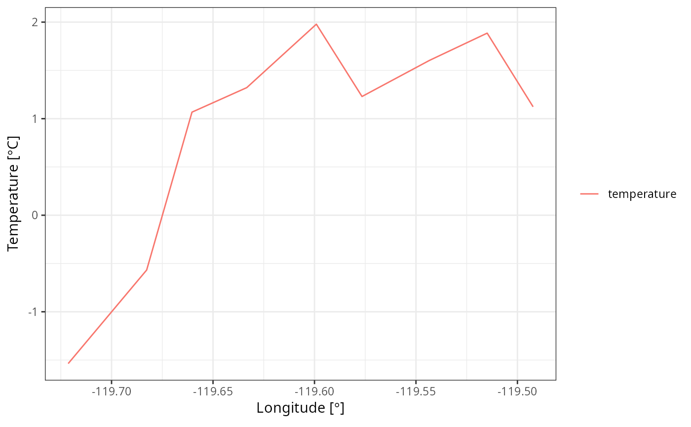
#> 6 1.321479  6 temperature -119.6334 38.75301 POINT (-119.6334 38.75301)

Add time variable, select and plot

library(ggplot2)
ggplot(df, 
       aes(x = X, y = V1, colour = V3)) +
  labs(y =expression(paste("Temperature [",degree,"C]")),
       x = expression(paste("Longitude [",degree,"]")))+
  geom_line() +
  theme_bw()+
  theme(legend.title = element_blank())

Sergio Ibarra-Espinosa

2024-09-22