EmissV is a R-package that provides tools to create emissions for use in numeric air quality models such as WRF-Chem. The package can read inputs from global fluxes from inventories in Netcdf Format [1] or estimate the emissions using top-down approach for point/line/area sources [2].
[1] Schuch D, Ibarra-Espinosa S, Dias de Freitas E, Andrade M (2018). “EmissV: A preprocessor for WRF-Chem model.” Journal of Atmospheric Science Research, 5, doi:10.30564/jasr.v1i1.347.
[2] Schuch D, Ibarra-Espinosa S, Dias de Freitas E (2018). “EmissV: An R package to create vehicular and other emissions by Top-down methods to air quality models.” The Journal of Open Source Software, 6, doi:10.21105/joss.00662.
Installation
System dependencies
EmissV import functions from ncdf4 for reading model information, raster and sf to process grinded/geographic information and units. These packages need some aditional libraries:
To Ubuntu
The following steps are required for installation on Ubuntu:
  sudo add-apt-repository ppa:ubuntugis/ubuntugis-unstable --yes
  sudo apt-get --yes --force-yes update -qq
  # netcdf dependencies:
  sudo apt-get install --yes libnetcdf-dev netcdf-bin
  # units/udunits2 dependency:
  sudo apt-get install --yes libudunits2-dev
  # sf dependencies (without libudunits2-dev):
  sudo apt-get install --yes libgdal-dev libgeos-dev libproj-dev
To Windows
No additional steps for windows installation.
Detailed instructions can be found at netcdf, libudunits2-dev and sf developers page.
To conda (miniconda / anaconda)
First create a new environment called rspatial (or a better name):
and to install some requisites:
Package installation
To install the CRAN version:
install.packages("EmissV")To install the development version using remotes:
or to install the development version using devtools:
require("devtools")
devtools::install_github("atmoschem/EmissV")
Using EmissV with EDGAR 8.1 emissions
EmissV can be used to process emissions of atmospheric pollutants and green house gases from inventories such as EDGAR, RCP, GAINS and other datasets in NetCDF format, the GEIA-ACCENT and ECCAD emission data portal makes available some of these inventories. You can verify the supported format with:
EmissV::read()To generate a simple emission it’s a straightforward process in 4 steps:
library(EmissV)
### 1. download the EDGAR 8.1 Netcdf flux file using R or from
### https://jeodpp.jrc.ec.europa.eu/ftp/jrc-opendata/EDGAR/datasets
# create the temporary directory to download the data
folder <- file.path(tempdir(), "EDGARv8.1")
dir.create(folder)
# download the total emissions of NOx from EDGAR v50_AP for 2015
url     <- "https://jeodpp.jrc.ec.europa.eu/ftp/jrc-opendata/EDGAR/datasets"
dataset <- "v81_FT2022_AP_new/NOx/TOTALS/flx_nc"
file    <- "v8.1_FT2022_AP_NOx_2022_TOTALS_flx_nc.zip"
download.file(paste0(url,"/",dataset,"/",file), paste0(folder,"/",file))
# unzip the file
unzip(paste0(folder,"/",file),exdir = folder)

### 2. read the emissions (using the spec argument to split NOx into NO and NO2)
nox  <- read(file    = dir(path=folder, pattern="flx\\.nc", full.names=TRUE),
             version = "EDGARv8",
             spec    = c(E_NO  = 0.9 ,   # 90% of NOx is NO
                         E_NO2 = 0.1 ))  # 10% of NOx is NO2

### 3. get the information from a WRF grid from a initial conditions file (wrfinput)
g   <- gridInfo(paste(system.file("extdata", package = "EmissV"),"/wrfinput_d01",sep=""))

### 4. calculate the emissions for grid g
NO  <- emission(grid = g, inventory = NOx$E_NO, pol = "NO", mm = 30.01,   plot = T)
NO2 <- emission(grid = g, inventory = NOx$E_NO2,pol = "NO2",mm = 46.0055, plot = T)
The next step is to save the emission in a emission file, the next example show how to save emissions using the eixport R-package:
library(eixport)
### create a temporary folder for emissions
dir.create(file.path(tempdir(), "EMISSION"))

### create the emision file
wrf_create(wrfinput_dir = system.file("extdata", package = "EmissV"),
           wrfchemi_dir = file.path(tempdir(), "EMISSION"),
           domains      = 1)

### get the file path of the emission file
emis_file <- list.files(path = file.path(tempdir(), "EMISSION"),
                        pattern = "wrfchemi_d01",
                        full.names = TRUE)

### save the emission
wrf_put(NO,  file = emis_file, name = "E_NO",  verbose = TRUE)
wrf_put(NO2, file = emis_file, name = "E_NO2", verbose = TRUE)
Check the wrf_create, wrf_put and to_wrf to more information and customize for your application.
NOTE: The emission file must be compatible with the WRF-Chem options (many arguments are the same as the namelist.input from WRF) check the eixport R-Package documentation and the WRF-Chem manual for more information.
Other R-packages are available to write netcdf such as ncdf4, RNetCDF, tidync are available on CRAN. Other languages such as NCL leanguage and the Python package wrf-python, and preprocessor anthro_emiss are aternative to write NetCDF files.
Using EmissV to estimate vehicular emissions
In EmissV the vehicular emissions are estimated by a top-down approach, i.e. the emissions are calculated using the statistical description of the fleet at avaliable level (National, Estadual, City, etc).The following steps show an example workflow for calculating vehicular emissions, these emissions are initially temporally and spatially disaggregated, and then distributed spatially and temporally.
I. Total: emission of pollutants is estimated from the fleet, use and emission factors and for the interest area (cities, states, countries, etc).
library(EmissV)

fleet <- vehicles(example = T)
# using a example of vehicles (DETRAN 2016 data and SP vahicle distribution):
#                              Category   Type Fuel      Use       SP ...
# Light Duty Vehicles Gasohol   LDV_E25    LDV  E25  41 km/d 11624342 ...
# Light Duty Vehicles Ethanol  LDV_E100    LDV E100  41 km/d   874627 ...
# Light Duty Vehicles Flex        LDV_F    LDV FLEX  41 km/d  9845022 ...
# Diesel Trucks               TRUCKS_B5 TRUCKS   B5 110 km/d   710634 ...
# Diesel Urban Busses           CBUS_B5    BUS   B5 165 km/d   792630 ...
# Diesel Intercity Busses       MBUS_B5    BUS   B5 165 km/d    21865 ...
# Gasohol Motorcycles          MOTO_E25   MOTO  E25 140 km/d  3227921 ...
# Flex Motorcycles               MOTO_F   MOTO FLEX 140 km/d   235056 ...

fleet <- fleet[,c(-6,-8,-9)] # dropping RJ, PR and SC

EF     <- emissionFactor(example = T)
# using a example emission factor (values calculated from CETESB 2015):
#                                     CO          PM
# Light duty Vehicles Gasohol  1.75 g/km 0.0013 g/km
# Light Duty Vehicles Ethanol 10.04 g/km 0.0000 g/km
# Light Duty Vehicles Flex     0.39 g/km 0.0010 g/km
# Diesel trucks                0.45 g/km 0.0612 g/km
# Diesel urban busses          0.77 g/km 0.1052 g/km
# Diesel intercity busses      1.48 g/km 0.1693 g/km
# Gasohol motorcycles          1.61 g/km 0.0000 g/km
# Flex motorcycles             0.75 g/km 0.0000 g/km

TOTAL  <- totalEmission(fleet,EF,pol = c("CO"),verbose = T)
# Total of CO : 1128297.0993334 t year-1
II. Spatial distribution: The package has functions to read information from tables, georeferenced images (tiff), shapefiles (sh), OpenStreet maps (osm), global inventories in NetCDF format (nc) to calculate point, line and area sources.
raster <- raster::raster(paste(system.file("extdata", package = "EmissV"),
                         "/dmsp.tiff",sep=""))

grid   <- gridInfo(paste(system.file("extdata", package = "EmissV"),
                   "/wrfinput_d02",sep=""))
# Grid information from: .../EmissV/extdata/wrfinput_d02

shape  <- raster::shapefile(paste(system.file("extdata", package = "EmissV"),
                            "/BR.shp",sep=""),verbose = F)[12,1]
Minas_Gerais <- areaSource(shape,raster,grid,name = "Minas Gerais")
# processing Minas Gerais area ...
# fraction of Minas Gerais area inside the domain = 0.0145921494236101

shape  <- raster::shapefile(paste(system.file("extdata", package = "EmissV"),
                            "/BR.shp",sep=""),verbose = F)[22,1]
Sao_Paulo <- areaSource(shape,raster,grid,name = "Sao Paulo")
# processing Sao Paulo area ...
# fraction of Sao Paulo area inside the domain = 0.474658563750987

sp::spplot(raster::merge(drop_units(TOTAL$CO[[1]]) * Sao_Paulo,
                         drop_units(TOTAL$CO[[2]]) * Minas_Gerais),
           scales = list(draw=TRUE),ylab="Lat",xlab="Lon",
           main=list(label="Emissions of CO [g/d]"),
           col.regions = c("#031638","#001E48","#002756","#003062",
                           "#003A6E","#004579","#005084","#005C8E",
                           "#006897","#0074A1","#0081AA","#008FB3",
                           "#009EBD","#00AFC8","#00C2D6","#00E3F0"))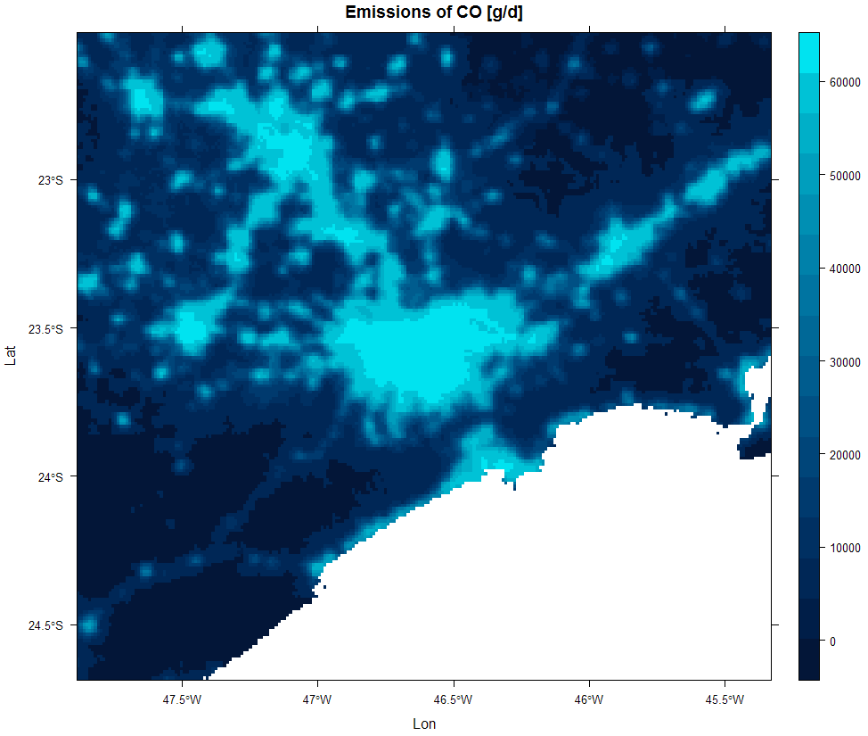
III. Emission calculation: calculate the final emission from all different sources and converts to model units and resolution.
CO_emissions <- emission(total = TOTAL,
                         pol   = "CO",
                         area  = list(SP = Sao_Paulo, MG = Minas_Gerais),
                         grid  = grid,
                         mm    = 28,
                         plot  = T)
# calculating emissions for CO using molar mass = 28 ...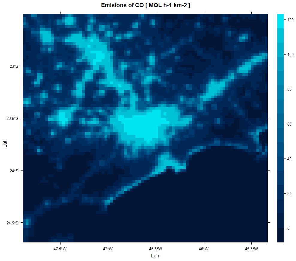
IV. Temporal distribution: the package has a set of hourly profiles that represent the mean activity for each day of the week calculated from traffic counts of toll stations located in São Paulo city.
The package has additional functions for read netcdf data, create line and point sources (with plume rise) and to estimate the total emissions of of volatile organic compounds from exhaust (through the exhaust pipe), liquid (carter and evaporative) and vapor (fuel transfer operations).
Functions:
- read: read global inventories in netcdf format
- vehicles: tool to set-up vehicle data.table
- emissionFactor: tool to set-up emission factors data.table
- gridInfo: read grid information from a NetCDF file
- pointSource: emissions from point sources
- plumeRise: calculate plume rise
- rasterSource: distribution of emissions by a georeferenced image
- lineSource: distribution of emissions by line vectors
- areaSource: distribution of emissions by region
- totalEmission: total emissions
- emission: Emissions to atmospheric models
- speciation: Speciation of emissions in different compounds
Sample datasets:
- Species: species mapping tables
- Perfil: vehicle counting profile for vehicular activity
- Sample of an image of persistent lights of the Defense Meteorological Satellite Program (DMSP)
- CETESB 2015 emission factors as
emissionFactor(example=T) - DETRAN 2016 data and SP vahicle distribution as
vehicles(example=T) - Shapefiles for Brazil states
Contributing
Bug reports, suggestions, and code contributions are all welcome. Please see CONTRIBUTING.md for details. Note that this project adopt the Contributor Code of Conduct and by participating in this project you agree to abide by its terms.
License
EmissV is published under the terms of the MIT License. Copyright (c) 2018 Daniel Schuch.